Cold junction compensation (CJC) is a method used with thermocouples to ensure accurate temperature measurements. Thermocouples generate a voltage based on the temperature difference between the hot and cold junctions. The cold junction, where the thermocouple wires are connected to the measurement device, needs to be accurately compensated for to avoid errors in temperature readings.
The most common way to compensate for the cold junction is by measuring its temperature using a direct-reading temperature sensor. This sensor provides a reference temperature that allows adjustments to be made to the temperature reading from the thermocouple, ensuring accuracy.
Another less common method involves forcing the junction between the thermocouple metal and copper metal to a known temperature, typically 0°C, by immersing it in an ice bath. Then, the copper wire from each junction is connected to a voltage measurement device to provide accurate temperature readings.
How Produce Cold Junction Compensation?
A thermocouple generates a voltage (thermoelectromotive force) due to the temperature difference between its hot and cold junctions. This voltage represents a relative temperature, not an absolute one. To determine the absolute temperature at the hot junction, the effect of the cold junction temperature must be compensated for. This is achieved by detecting the cold junction temperature and adding a corresponding thermoelectromotive force to that of the thermocouple. This process, known as cold junction compensation, allows the Temperature Controller to calculate the absolute temperature of the hot junction accurately.
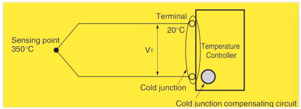
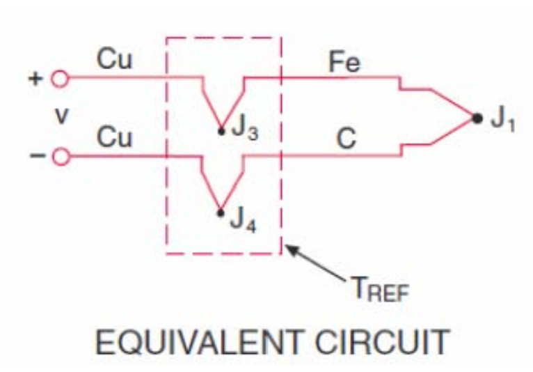
In the provided diagram, the thermoelectromotive force (V_T) measured at the Temperature Controller’s input terminal equals (V(350, 20)), where (V(A, B)) represents the thermoelectromotive force when the cold junction is at (A) °C and the hot junction is at (B) °C.
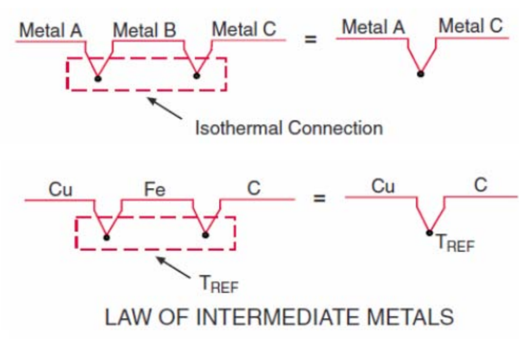
According to the law of intermediate temperatures, a fundamental property of thermocouples states that (V(A, B) = V(A, C) – V(B, C)), where (C) represents the temperature of the cold junction.
Basics of Cold Junction Compensation
Thermocouple temperature measurements involve two key elements: measuring the thermal gradient using the thermocouple’s output based on the Seebeck effect, and measuring the temperature at the cold junction. The output coefficient of a thermocouple is typically a few microvolts per degree Celsius. For high-accuracy systems, precise processing blocks with high resolution are needed to effectively resolve microvolt-level signals.
Alternatively, the thermocouple output can be amplified using a low-noise, low-offset amplifier. This approach simplifies the system complexity for subsequent stages. The amplifier’s gain can be adjusted to match the required temperature measurement range.
Accurate measurement of the cold junction temperature is crucial because any error is directly added to the temperature gradient and cannot be corrected. Cold junction temperature measurements can be accomplished using various methods such as local diodes, resistance temperature detectors (RTDs), thermistors, or device-based temperature sensors. RTDs and thermistors require excitation sources and additional signal processing, while diode-based sensors have limited linearity over a small temperature range. Device-based sensors are preferred due to their linear output, relatively low cost, and high accuracy, typically with a slope of around 5 mV/ºC or 10 mV/ºC.
A measurement system equipped with an analog-to-digital converter (ADC) and controller can capture both the thermocouple amplified signal and the cold junction signal. The controller can then handle the different slopes of these signals in software to calculate the cold-junction compensated temperature gradient and, consequently, the temperature at the hot junction.
In some cases, performing cold junction compensation in the analog domain may be necessary due to various system constraints, such as limitations with the ADC or available channels, software overheads, system complexity, and cost considerations.
Figure 3 provides a method to achieve the required output voltage for a specific temperature range. Section 3 guides the design of component values based on factors like output range, temperature range, thermocouple type, etc. Section 3.2 elaborates on the design calculations. Calculated values can be applied to Figure 3 to validate the design.
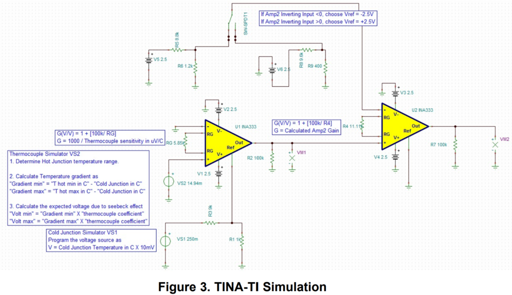
The design employs a two-stage approach, with each stage utilizing an instrumentation amplifier (INA) known for low offset at high gains, minimal offset drift, and low noise. One example is the INA333 from Texas Instruments, which operates within a supply voltage range of up to 5 V. For larger output voltage swings, an INA with higher supply voltage capability should be selected.
For cold junction temperature measurement, an integrated circuit (IC)-based analog output device like the LM35 is chosen. The LM35 offers linear output with a slope of 10 mV/ºC.
The TINA-TI simulation design depicted in Figure 3 implements the cold-junction compensation method described in this application note. The TINA simulation design is accessible at SBOC445. In the final design, VS2 represents the chosen thermocouple, while VS1 represents a cold-junction measurement device like the LM35. V5 and V6 serve as positive and negative references for stage 2.
Law of Intermediate Metals
CJC and J Type Thermocouple